Chemical Structure Alignment
Molecular alignment is a fundamental problem in cheminformatics and can be used for structure determination, similarity based searching, and ligand-based drug design. This problem can be formulated as an orthogonal Procrustes problem where the two matrices represent three-dimensional Cartesian coordinates of molecules.
Orthogonal Procrustes
Given matrix \(\mathbf{A}_{m \times n}\) and a reference \(\mathbf{B}_{m \times n}\), find the find the orthogonal transformation matrix \(\mathbf{Q}_{n \times n}\) that makes \(\mathbf{A}\) as close as possible to \(\mathbf{B}\), i.e.,
\begin{equation} \underbrace{\min}_{\left\{\mathbf{Q} | \mathbf{Q}^{-1} = {\mathbf{Q}}^\dagger \right\}} \|\mathbf{A}\mathbf{Q} - \mathbf{B}\|_{F}^2 \end{equation}
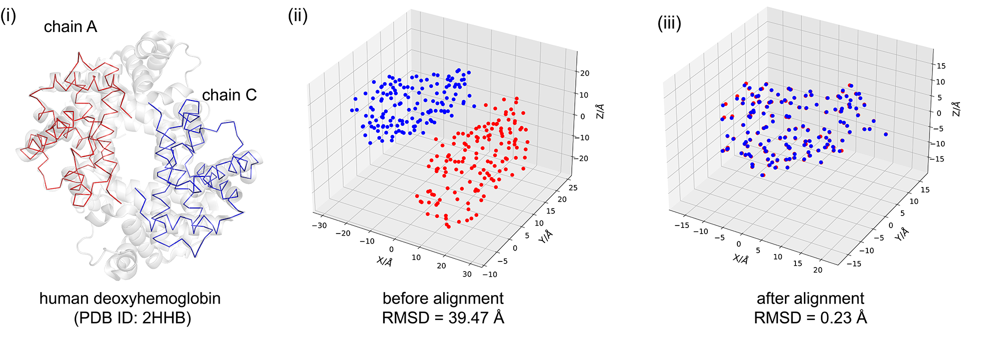
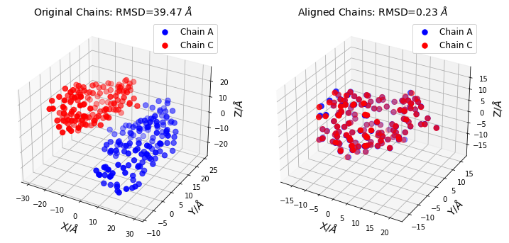
In the code block below, we use the procrustes library for protein structure alignment. We use the 2HHB, which has cyclic-\(C_2\) global symmetry, and load its PDB file using IOData library to obtain the 3D-Cartesian coordinates atoms. In 2HHB, the A and C (or B and D) are hemoglobin deoxy-alpha (beta) chains shown in Fig. (i), and their \(C_{\alpha}\) atoms in Fig. (ii) are aligned in Fig. (iii) to show that they are homologous.
The results in Fig. (iii) are obtained with orthogonal Procrustes which implements the Kabsch algorithm. The root-mean-square deviation (RMSD) is used to assess the discrepancy between structures before and after the translation-rotation transformation.
Download IOData & Matplotlib Libraries & Example Files
Install IOData library and Matplotlib, if there are not available on your system; this is required on Binder.
Download 2hhb.pdb file used in the example below which is stored in Procrustes GitHub repository example files.
[ ]:
# If needed, install IOData library (this is required on Binder)

import sys

# See https://jakevdp.github.io/blog/2017/12/05/installing-python-packages-from-jupyter/
!{sys.executable} -m pip install qc-iodata
!{sys.executable} -m pip install matplotlib
[ ]:
# If needed, download the example files
import os
from urllib.request import urlretrieve

fpath = "notebook_data/chemical_strcuture_alignment/"
if not os.path.exists(fpath):
    os.makedirs(fpath, exist_ok=True)

urlretrieve(
    "https://raw.githubusercontent.com/theochem/procrustes/master/doc/notebooks/notebook_data/chemical_strcuture_alignment/2hhb.pdb",
    os.path.join(fpath, "2hhb.pdb")
    )
Procrustes Analysis
[1]:
# chemical structure alignment with orthogonal Procrustes
from pathlib import Path

import numpy as np
from iodata import load_one
from iodata.utils import angstrom
from procrustes import rotational

# load PDB
pdb = load_one(Path("notebook_data/chemical_strcuture_alignment/2hhb.pdb"))

# get coordinates of C_alpha atoms in chains A & C (in angstrom)
chainid = pdb.extra['chainids']
attypes = pdb.atffparams['attypes']
# alpha carbon atom coordinates in chain A
ca_a = pdb.atcoords[(chainid == 'A') & (attypes == 'CA')] / angstrom
# alpha carbon atom coordinates in chain A
ca_c = pdb.atcoords[(chainid == 'C') & (attypes == 'CA')] / angstrom

# compute root-mean-square deviation of original chains A and C
rmsd_before = np.sqrt(np.mean(np.sum((ca_a - ca_c)**2, axis=1)))
print("RMSD of initial coordinates:", rmsd_before)

# rotational Procrustes analysis
result = rotational(ca_a, ca_c, translate=True)

# compute transformed (translated & rotated) coordinates of chain A
ca_at = np.dot(result.new_a, result.t)

# compute root-mean-square deviation of trainsformed chains A and C
rmsd_after = np.sqrt(np.mean(np.sum((ca_at - result.new_b)**2, axis=1)))
print("RMSD of transformed coordinates:", rmsd_after)
RMSD of initial coordinates: 39.46851987559469
RMSD of transformed coordinates: 0.23003870483785113
Plot Procrustes Results
[2]:
# Plot outputs of Procrustes

import matplotlib.pyplot as plt

fig = plt.figure(figsize=(12, 10))

# =============
# First Subplot
# =============
# set up the axes for the first plot
ax = fig.add_subplot(1, 2, 1, projection='3d')

# coordinates of chains A & C (before alignment)
coords1, coords2 = ca_a, ca_c
title = "Original Chains: RMSD={:0.2f} $\AA$".format(rmsd_before)

ax.scatter(xs=coords1[:, 0], ys=coords1[:, 1], zs=coords1[:, 2],
           marker="o", color="blue", s=55, label="Chain A")
ax.scatter(xs=coords2[:, 0], ys=coords2[:, 1], zs=coords2[:, 2],
           marker="o", color="red", s=55, label="Chain C")

ax.set_xlabel("X/$\AA$", fontsize=14)
ax.set_ylabel("Y/$\AA$", fontsize=14)
ax.set_zlabel("Z/$\AA$", fontsize=14)
ax.legend(fontsize=12, loc="best")
plt.title(title, fontsize=14)


# ==============
# Second Subplot
# ==============
# set up the axes for the second plot
ax = fig.add_subplot(1, 2, 2, projection='3d')

# coordinates of chains A & C after translation and rotation
coords1, coords2 = ca_at, result.new_b
title="Aligned Chains: RMSD={:0.2f} $\AA$".format(rmsd_after)

ax.scatter(xs=coords1[:, 0], ys=coords1[:, 1], zs=coords1[:, 2],
           marker="o", color="blue", s=55, label="Chain A")
ax.scatter(xs=coords2[:, 0], ys=coords2[:, 1], zs=coords2[:, 2],
           marker="o", color="red", s=55, label="Chain C")

ax.set_xlabel("X/$\AA$", fontsize=14)
ax.set_ylabel("Y/$\AA$", fontsize=14)
ax.set_zlabel("Z/$\AA$", fontsize=14)
ax.legend(fontsize=12, loc="best")
plt.title(title, fontsize=14)

plt.show()
The corresponding file can be obtained from:
Jupyter Notebook:
Chemical_Structure_Alignment.ipynbInteractive Jupyter Notebook:
